Depending on the complexity of your SQL query there are many, often exponential, query plans that return the same result. However, the performance of each plan can vary drastically; taking only seconds to finish or days given the chosen plan.

That places a significant burden on analysts who will then have to know how to write performant SQL. This problem gets worse as the complexity of questions and SQL queries increases. In the absence of an optimizer, queries will be executed with syntactic ordering in the way the query was written. That’s a burden that isn’t reasonable to place on a group of users who know what questions need answering but who aren’t, and shouldn’t have to be, wizards with SQL. An analyst should be able to submit a query and get a fast result without having to worry about how to optimally structure the question in SQL.

With this problem in mind, developers at Starburst developed Trino’s first Cost-Based Optimizer (CBO). Packaged alongside the 195e release (and higher), the CBO’s primary job is to explore the space of possible query plans and to find the most optimal. The CBO removes the burden from the end user of knowing how to write performant SQL.

The Cost-Based Optimizer (CBO) has shown impressive results in industry standard benchmarks since its release in early April 2018, claiming speeds up to 13 times faster than the competition. Thanks to its extensive decision-making process, based on the shape of the query, filters, and table statistics, the CBO can evaluate and execute the most optimal query plan among the countless alternatives.

Background

An analysis of the CBO and its methods of statistical analyses first require a contextual framework. Let’s consider a data scientist who wants to understand which of the company’s customers spend the most money. They submit a query similar to that below.

     SELECT c.custkey, sum(l.price)
     FROM customer c, orders o, lineitem l
     WHERE c.custkey = o.custkey AND l.orderkey = o.orderkey
     GROUP BY c.custkey
     ORDER BY sum(l.price) DESC;

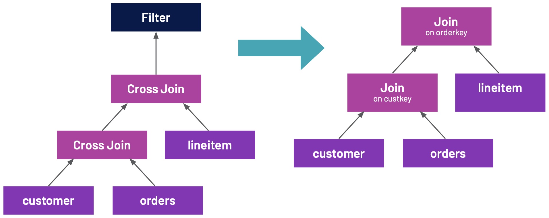
Once the above query is put into action, Trino must create a plan for its execution. It does so by first transforming the query into its simplest possible plan. It will create CROSS JOINS for the “FROM customer c, orders o, lineitem l” part of the query and FILTER for “WHERE c.custkey = o.custkey AND l.orderkey = o.orderkey”. This initial plan is quite naïve, as CROSS JOINS will produce humongous amounts of intermediate data. In fact, there is no point in even trying to execute such a plan, and Trino never does. Instead, it transforms the plan to create one more in line with the user’s expectations, as shown below.

Note: for succinctness, only part of the query plan is drawn, without aggregation (“GROUP BY”) and sorting (“ORDER BY”).

如果想及时了解Spark、Hadoop或者HBase相关的文章，欢迎关注微信公众号：iteblog_hadoop

Indeed, this is much better than the original CROSS JOINS plan. Yet still, a more optimal execution plan can be reached if costs are considered.

Cost-Based Optimizer

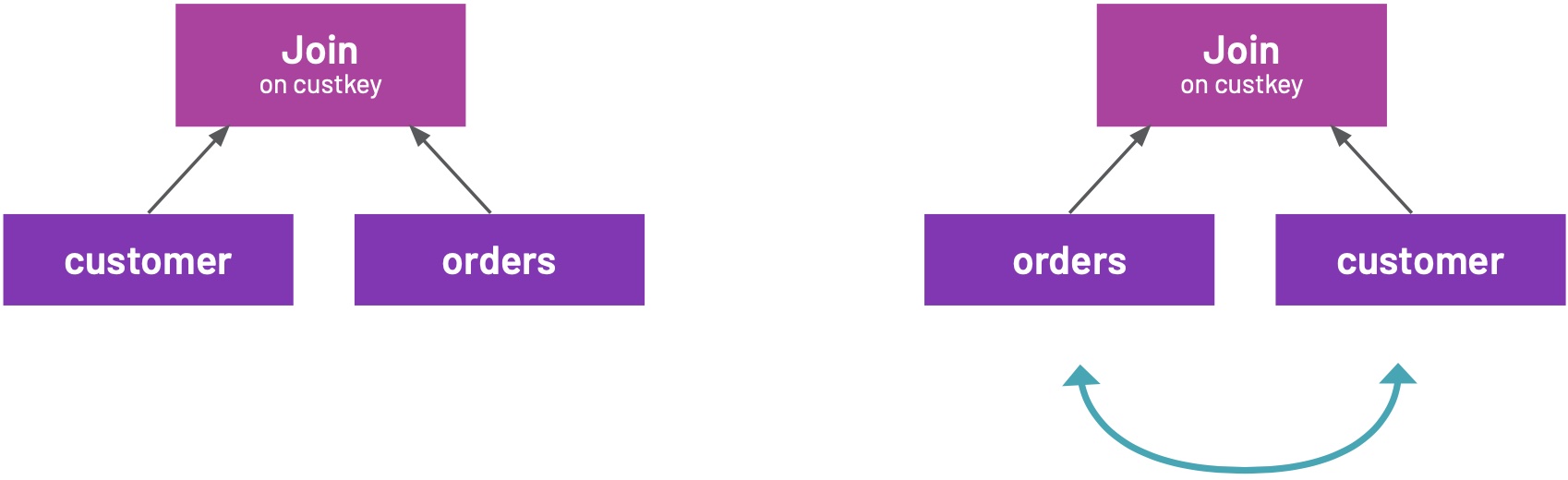
Without going into database internals on how JOIN is implemented, it is important to understand
that it makes a big difference which table is right and which is left in the JOIN; the simple explanation being that the table on the right needs to be kept in the memory while the JOIN result is calculated. Consequently, the following plans produce the same result but have potentially different execution time or memory requirements.

如果想及时了解Spark、Hadoop或者HBase相关的文章，欢迎关注微信公众号：iteblog_hadoop

CPU time, memory requirements, and network bandwidth usage are the three dimensions that contribute to query execution time, both in a single query and concurrent workloads. These dimensions capture the “cost” or overall efficiency of each query plan. Thus, it is important to consider the position and size of the tables within your JOIN in order to limit the cost of your query.

Say our data scientist knows that most of the customers made at least one order, that each of those orders had at least one item, and that many orders had many items. They would then know that “lineitem” is the biggest table, “orders” is the medium table and “customer” is the smallest table. When joining “customer” and “orders” in this case, they would put “orders” on the left side of the JOIN and “customer” on the right, as customer is the smaller table. But the query planner cannot be cognizant of such information for every query they submit. In reality, the planner cannot reliably deduce information from table names alone; for this, statistics are needed.

Table Statistics

It is important to understand that Trino has a connector-based architecture, and such connectors can provide table and column statistics:

• Number of rows in a table
• Number of distinct values in a column
• Fraction of NULL values in a column
• Minimum/maximum value in a column
• Average data size for a column

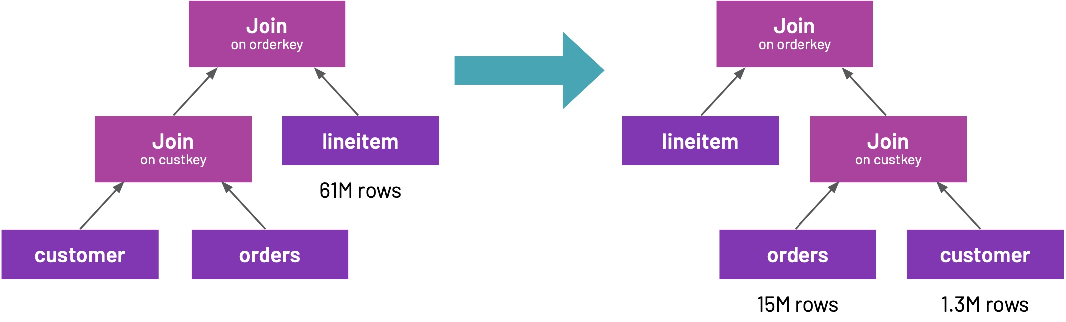
And so, if some information is missing — the average text length in a varchar column for example — a connector can still provide information in which the Cost-Based Optimizer can take advantage. In our data scientist’s example, data sizes can look something like the following:

如果想及时了解Spark、Hadoop或者HBase相关的文章，欢迎关注微信公众号：iteblog_hadoop

Having this knowledge, Trino’s Cost-Based Optimizer will think up a completely different JOIN ordering in the query plan.

如果想及时了解Spark、Hadoop或者HBase相关的文章，欢迎关注微信公众号：iteblog_hadoop

Filter Statistics

As we saw, knowing the sizes of the tables involved in a query is critical to reordering JOINs properly in the query plan. However, knowing just the sizes is not enough. Returning to our example, consider the data scientist wants to understand which customers repeatedly spent the most money on a particular item. For this, they will use a query almost identical to the original, but with the addition of the bolded condition below.

     SELECT c.custkey, sum(l.price)
     FROM customer c, orders o, lineitem l
     WHERE c.custkey = o.custkey AND l.orderkey = o.orderkey
          AND l.item = 106170
     GROUP BY c.custkey ORDER BY sum(l.price) DESC;

The additional FILTER could be applied after the JOIN or before. However, filtering as early as possible is the best strategy, as it reduces the amount of data you are working with from the beginning. In this case, the actual size of the data involved in the JOIN will be smaller. This can also alter the order in which your JOIN is executed, as shown in our data scientist’s example.

如果想及时了解Spark、Hadoop或者HBase相关的文章，欢迎关注微信公众号：iteblog_hadoop

Execution Time and Cost

From an external perspective, only three things matter when it comes to query optimization:

• Execution Time: The execution time is often called “wall time” to emphasize that we’re not really interested in “CPU time” or the number of machines, nodes, or threads involved.
• Execution Cost: The execution cost is the actual cost in dollars of running the query. A CFO will be most interested in this metric, as keeping cluster costs as low as possible is a large priority.
• Concurrent Queries: A check for concurrent queries ensures that all cluster users can work at the same time. That is, that the cluster can handle many queries at a time, yielding enough throughput that “wall time” observed by each of the users is satisfactory.

如果想及时了解Spark、Hadoop或者HBase相关的文章，欢迎关注微信公众号：iteblog_hadoop

It is only possible to optimize for one of the above dimensions. For example, you can have a single node cluster which would mitigate execution costs but drive up execution times and leave workers waiting idly. Contrarily, we may have a thousand-node cluster that cuts down execution times, but greatly increases execution costs for the organization. Ultimately, such tradeoffs must be balanced, such that queries are executed as fast as possible, with as little resources as possible.

In Trino, this is modeled with the concept of cost, which captures properties like CPU cost, memory requirements, and network bandwidth usage. In search of the most optimal solution, different variants of a query execution plan are explored, assigned a cost, and compared. Then, the variant with the least overall cost is selected for execution. This approach neatly balances the needs of each party - cluster users, administrators, and the CFO.

The cost of each operation in the query plan is calculated with the type of the operation in mind, taking into account the statistics of the data involved. Now, let’s see where the statistics come from.

Statistics

In our data scientist’s example, the row counts for tables were taken directly from table statistics, i.e., provided by a connector. But where did “~3K rows” come from? Let’s take a deeper dive into some of these details.

A query execution plan is made of “building block” operations, including:

• Table scans (reading the table; at runtime this is actually combined with a FILTER)
• FILTERs (SQL’s WHERE clause or any other conditions deduced by the query planner)
• Projections (i.e., computing output expressions)
• JOINs
• Aggregations (in fact there are a few different “building blocks” for aggregations, but that’s a story for another time)
• Sorting (SQL’s ORDER BY)
• Limiting (SQL’s LIMIT)
• Sorting and limiting combined (SQL’s ORDER BY .. LIMIT .. deserves specialized support)
• ETC.

The process by which these statistics are computed for such “building blocks” is discussed on the next page.

如果想及时了解Spark、Hadoop或者HBase相关的文章，欢迎关注微信公众号：iteblog_hadoop

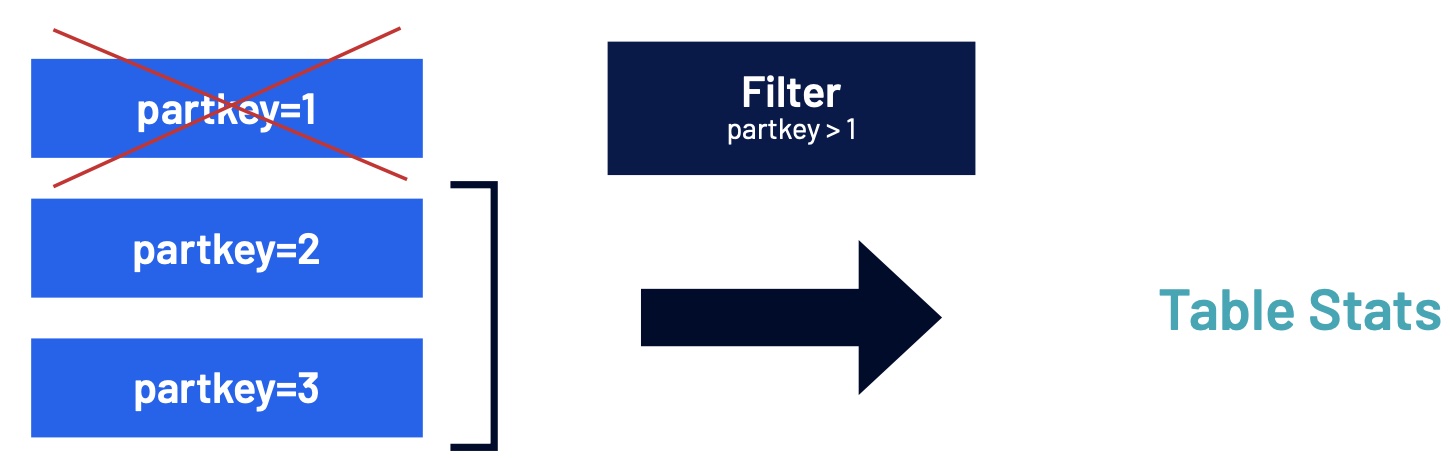
As explained earlier, the connector which defines the table is responsible for providing the table statistics. Further, the connector is informed of any filtering conditions that are to be applied to the data read from the table. This may be important in the case of a Hive partitioned table for example, where statistics are stored on a per-partition basis. If the filtering condition excludes some or many partitions, the statistics will consider a smaller data set (remaining partitions) and will be more accurate.
To recall, a connector can provide the following table and column statistics:

• Number of rows in a table,
• Number of distinct values in a column
• Fraction of NULL values in a column
• Minimum/maximum value in a column
• Average data size for a column
• ETC.

Filter Statistics

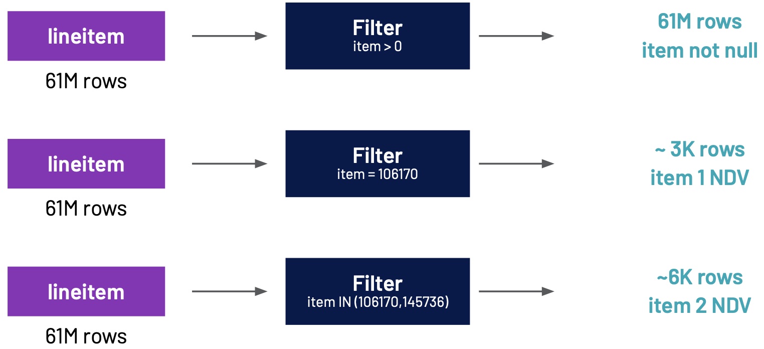
When considering a filtering operation, a filter’s condition is analyzed, and the following estimations are calculated:

• What is the probability that the data row will pass the filtering condition? From this, the expected number of rows after the filter is derived
• Fraction of NULL values for columns involved in the filtering condition (for many conditions, this will simply be 0%),
• Number of distinct values for columns involved in the filtering condition
• Number of distinct values for columns that were not part of the filtering condition, if their original number of distinct values was more than the expected number of data rows that pass the filter

For example, for a condition like “l.item = 106170” we can observe that:

• No rows with “l.item” being NULL will meet the condition
• There will be only one distinct value of “l.item” (106170) after the filtering operation
• On average, number of data rows expected to pass the filter will be equal to the number_of_input_rows * fraction_of_non_nulls / distinct_values. (This assumes, of course, that users most often drill down in the data they really have, which is quite a reasonable and safe assumption to make.)

如果想及时了解Spark、Hadoop或者HBase相关的文章，欢迎关注微信公众号：iteblog_hadoop

Projection Statistics

如果想及时了解Spark、Hadoop或者HBase相关的文章，欢迎关注微信公众号：iteblog_hadoop

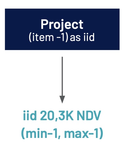
Projections (“l.item – 1 AS iid”) are similar to filters, except that they do not impact the expected number of rows after the operation.

For a projection, the following types of column statistics are calculated (if possible for the given projection expression):

• Number of distinct values produced by the projection
• Fraction of NULL values produced by the projection
• Minimum/maximum value produced by the projection

Naturally, if “iid” is only returned to the user, then these statistics are not useful. However, if it’s later used in a FILTER or JOIN operation, these statistics are important to the proper estimation of the number of rows that meet the FILTER condition or are returned from the JOIN.