在本文中,我将分享一些关于如何编写可伸缩的 Apache Spark 代码的技巧。本文提供的示例代码实际上是基于我在现实世界中遇到的。因此,通过分享这些技巧,我希望能够帮助新手在不增加集群资源的情况下编写高性能 Spark 代码。
背景
我最近接手了一个 notebook ,它主要用来跟踪我们的 AB 测试结果,以评估我们的推荐引擎的性能。这个 notebook 里面的代码运行起来非常的慢,以下代码片段(片段1)是运行时间最长的:
val df = bucketPeriod.map{date =>
	val Array(year, month, day) = date.split("-")
	getAnalytics(BucketRecSysTracking, Brand, year, month, day)
	.select("c1", "c2", "c3", "c4", "c5", "c6", "c7", "c8", "c9",
			"c10", "c11", "c12", "c13", "c14", "c15")
	.filter($"c3".isin(18, 37))
	.distinct
}.filter(_.count > 0)
.reduce(_ union _)
.cache
在我们的 AB 测试实验中,用于跟踪数据的文件按年、月和日划分到不同文件夹中,文中中每一行都是一个 JSON 字符串,每天可能有几百个 JSON 文件。如果上面代码中的 bucketPeriod 代表需要查询的天列表,那么对于每天的数据会调用 getAnalytics 函数去遍历每天对应的文件夹下面的 json 文件,程序得到了每天的统计数,然后通过 reduce(_ union _) 合并成一个 DataFrame,并且删掉了 c3 不满足 isin(18, 37) 的数据。
运行上面的代码来遍历三天的数据居然要花费 17.72 分钟,而运行 df.count 居然花费了 26.71 分钟!现在让我们来看看是否不通过增加机器的资源来加快运行速度。
在我们深入讨论之前,下来看一下 getAnalytics 函数的实现(片段2)。其主要作用就是读取某个目录下的所有 JSON 文件,然后根据一些字段的情况添加一些东西而已。
def getAnalytics(bucketName: String, brand: String, bucketYear: String, bucketMonth: String,
      bucketDay: String, candidate_field: String=candidateField, groups: String=Groups): DataFrame = {
  var rankingOrderedIds = Window.partitionBy("c12").orderBy("id")
  val s3PathAnalytics = getS3Path(bucketName, brand, bucketFolder, year=bucketYear, month=bucketMonth, day=bucketDay)
  readJSON(s3PathAnalytics)
    .distinct
    .withColumn("x", explode($"payload"))
    // a few more calls to withColumn to create columns
    .withColumn("c10", explode(when(size(col("x1")) > 0, col("x1")).otherwise(array(lit(null).cast("string")))))
    // a few more calls to withColumn to create columns
    .withColumn("id", monotonically_increasing_id)
    // a few more calls to withColumn to create columns
    .withColumn("c12", concat_ws("X", $"x2", $"x3", $"c3"))
    .withColumn("c13", rank().over(rankingOrderedIds))
    .distinct
}
技巧一:尽可能给 Spark 函数更多的输入路径
最上面的代码片段每次调用 spark.read.json 的时候只输入一个目录,这样的写法非常的低效,因为 spark.read.json 可以接受文件名列表,然后 driver 只需要调度一次就可以获取到这些文件列表里面的数据,而不是像上面一样每个路径调用一次。
所以如果你需要读取分散在不同文件夹里面的文件,你需要将类似于下面的代码(片段3)
getDays("2019-08-01", "2019-08-31")
	.map{date =>
		val Array(year, month, day) = date.split("-")
	  	val s3PathAnalytics = getS3Path(bucketName, brand, bucketFolder, bucketYear, bucketMonth, bucketDay)
  		readJSON(s3PathAnalytics)
	}
修改成以下的代码逻辑(片段4)
val s3Files = getDays("2019-08-01", "2019-08-31")
				.map(_.split("-"))
				.map{
					case Array(year, month, day) => getS3Path(bucketName, brand, bucketFolder, bucketYear, bucketMonth, bucketDay)
				}

spark.read.json(s3Files: _*)
这样的写法比之前的写法速度是要快的,而且如果输入的目录越多,速度也要更快。
技巧二:尽可能跳过模式推断
根据 spark.read.json 文档的描述:spark.read.json 函数会先遍历一下输入的目录,以便确定输入数据的 schema。所以如果你事先知道输入文件的 schema,最好事先指定。
因此,我们的代码可以修改成以下样子(片段5):
val s3Files = getDays("2019-08-01", "2019-08-31")
				.map(_.split("-"))
				.map{
					case Array(year, month, day) => getS3Path(bucketName, brand, bucketFolder, bucketYear, bucketMonth, bucketDay)
				}

val jsonString = spark.read.json(s3Files(0)).schema.json
val newSchema = DataType.fromJson(jsonString).asInstanceOf[StructType]

spark.read.schema(newSchema).json(s3Files: _*)
上面代码片段我们先扫描了第一个文件,然后从文件中获取了数据的 schema,然后把获取到的 schema 传递给 spark.read,上面的代码片段一共运行了 29.82。
技巧三:尽可能避免 Shuffle
现在我们已经提高了文件 I/O 的速度,让我们来看看能不能提升 getAnalytics 函数的运行速度。
getAnalytics 函数里面一开始就调用了 distinct,这个是会导致 shuffle 的算子。那我们如何快速识别出哪些操作会导致 shuffle 呢?答案是调用 RDD 函数上面的 toDebugString 函数,即可判断,具体如下:
df1.distinct.rdd.toDebugString

res20: String =
(200) MapPartitionsRDD[951] at rdd at command-1:1 []
  |	  MapPartitionsRDD[950] at rdd at command-1:1 []
  |	  MapPartitionsRDD[949] at rdd at command-1:1 []
  |	  ShuffledRowRDD[948] at rdd at command-1:1 []
  +-(350) MapPartitionsRDD[947] at rdd at command-1:1 []
  	  |   MapPartitionsRDD[946] at rdd at command-1:1 []
  	  |   FileScanRDD[945] at rdd at command-1:1 []
使用同样的方法,我们也可以快速找到 rank().over(rankingOrderedIds) 方法也会导致 shuffle。
在这种情况下,读取文件后立即触发一次 shuffle 是一个坏主意,因为整个数据集是非常大的,而且我们可能还读出不需要的列。因此,我们不必在集群中移动这些大文件。我们要尽可能将 shuffle 的发生时间推到最后,而且最好先过滤一部分数据。
根据这些思路,我们可以将 getAnalytics 函数的实现重写如下(片段6):
val df2 = df1
    .withColumn("x", explode($"payload"))
    // a few more calls to withColumn to create columns
    .withColumn("c10", explode(when(size(col("x1")) > 0, col("x1")).otherwise(array(lit(null).cast("string")))))
    // a few more calls to withColumn to create columns
    .withColumn("id", monotonically_increasing_id)
    // a few more calls to withColumn to create columns
    .withColumn("c12", concat_ws("X", $"x2", $"x3", $"c3"))
    .withColumn("c13", rank().over(rankingOrderedIds))
    .select("c1", "c2", "c3", "c4", "c5", "c6", "c7", "c8", "c9",
			"c10", "c11", "c12", "c13", "c14", "c15")
	.filter($"c3".isin(18, 37))
	.distinct
为了清楚起见,我将片段1的相关代码部分合并到片段6中,以便得到相同的结果。注意,最开始的写法需要调用三次 distinct (一次在片段1,二次在片段2中),而最新的写法只需要调用一次 distinct,并得到同样的结果。当发生 shuffle 时(片段6中的第9行),物理计划显示只有 select 调用中指定的列被移动,这很好,因为它只是原始数据集中所有列的一个小子集。
片段6中的代码执行只花了0.90秒,count 只需要2.58分钟。这个例子表明,认真考虑我们编写好的查询是有好处的,这样可以避免执行一些不必要的 shuffle 操作。
技巧四:不要过度依赖 Catalyst Optimizer
我们比较以下两个代码片段:
val df2 = df1
    .withColumn("x", explode($"payload"))
    // a few more calls to withColumn to create columns
    .withColumn("c10", explode(when(size(col("x1")) > 0, col("x1")).otherwise(array(lit(null).cast("string")))))
    // a few more calls to withColumn to create columns
    .withColumn("id", monotonically_increasing_id)
    // a few more calls to withColumn to create columns
    .withColumn("c12", concat_ws("X", $"x2", $"x3", $"c3"))
    .withColumn("c13", rank().over(rankingOrderedIds))
    .select("c1", "c2", "c3", "c4", "c5", "c6", "c7", "c8", "c9",
			"c10", "c11", "c12", "c13", "c14", "c15")
	.filter($"c3".isin(18, 37))
	.distinct
以及
val df2 = df1
    .withColumn("x", explode($"payload"))
    // a few more calls to withColumn to create columns
    .withColumn("c10", explode(when(size(col("x1")) > 0, col("x1")).otherwise(array(lit(null).cast("string")))))
    // a few more calls to withColumn to create columns
    .withColumn("id", monotonically_increasing_id)
    // a few more calls to withColumn to create columns
    .withColumn("c12", concat_ws("X", $"x2", $"x3", $"c3"))
    .filter($"c3".isin(18, 37))
    .withColumn("c13", rank().over(rankingOrderedIds))
    .select("c1", "c2", "c3", "c4", "c5", "c6", "c7", "c8", "c9",
			"c10", "c11", "c12", "c13", "c14", "c15")
    .distinct
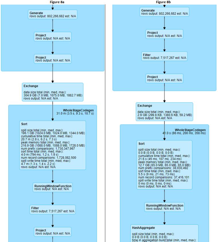
代码片段7和片段8功能是相同的,除了执行 fliter 的顺序不一样(分别是第14行和第9行)。但是这两个代码片段最后的输出结果是一样的,因为 rank 窗口函数并不用于 c3 这列,所以在执行 rank 之前或之后执行 filter 并不重要。但是,执行 df2.count 的时间有显著差异:片段7代码执行 df2.count 的时间为 2.58分钟,而片段8代码执行 df2.count 的时间为45.88秒。
这两个查询的物理计划解释了原因:
如果想及时了解Spark、Hadoop或者HBase相关的文章,欢迎关注微信公共帐号:iteblog_hadoop
上图显示,在调用 rank 窗口函数之前进行过滤的效果是将第一阶段的行数从 8.02 亿减少到仅仅700万。因此,当发生 shuffle 时,只需要在集群中移动 2.9 GB的数据。相反,在调用 rank 窗口函数之前没有进行过滤会导致 304.9 GB的数据在集群中移动。
这个例子告诉我们,如果您的查询中有 shuffle 操作,请仔细分析能不能先执行一些 filter 操作,以减少需要传输的数据量。另外,我们也要学会从物理计划中寻找一些优化点,而不能完全依赖于 Catalyst Optimizer,因为 Catalyst Optimizer 不是万能的。
本博客文章除特别声明,全部都是原创!原创文章版权归过往记忆大数据(过往记忆)所有,未经许可不得转载。
本文链接: 【Apache Spark 中编写可伸缩代码的4个技巧】(https://www.iteblog.com/archives/9731.html)